Note
Click here to download the full example code
Stack and Crop Raster Data Using EarthPy
Learn how to stack and crop satellite imagery using EarthPy
Stack and Crop Raster Data Using EarthPy
Note
The examples below will show you how to use the es.stack() and
es.crop_image() functions from EarthPy.
Stack Multi Band Imagery
Some remote sensing datasets are stored with each band in a separate file. However,
often you want to use all of the bands together in your analysis. For example
you need all of the bands together in the same file or “stack” in order to plot a color
RGB image. EarthPy has a stack() function that allows you
to take a set of .tif files that are all in the same spatial extent, CRS and resolution
and either export them together a single stacked .tif file or work with them in Python
directly as a stacked numpy array.
To begin using the EarthPy stack() function, import the needed packages
and create an array to be plotted. Below you plot the data as continuous with a colorbar
using the plot_bands() function.
Import Packages
You will need several packages to stack your raster. You will use GeoPandas to open up a shapefile that will be used to crop your data. You will primarily be using the EarthPy spatial module in this vignette.
import os
from glob import glob
import matplotlib.pyplot as plt
import rasterio as rio
from rasterio.plot import plotting_extent
import geopandas as gpd
import earthpy as et
import earthpy.spatial as es
import earthpy.plot as ep
Get Example Data Ready for Stack
With EarthPy you can create a stack from all of the Landsat .tif files (one per band)
in a folder with the es.stack() function.
Error found on Windows systems
Note
If you are running this script on a Windows system, there is a
known bug with .to_crs(), which is used in this script. If an error
occurs, you have to reset your os environment with the command
os.environ["PROJ_LIB"] = r"path-to-share-folder-in-environment".
# Get sample data from EarthPy and setting your home working directory

data_path = et.data.get_data("vignette-landsat")
os.chdir(os.path.join(et.io.HOME, "earth-analytics"))

# Prepare the landsat bands to be stacked using glob and sort

landsat_bands_data_path = "data/vignette-landsat/LC08_L1TP_034032_20160621_20170221_01_T1_sr_band*[2-4]*_crop.tif"
stack_band_paths = glob(landsat_bands_data_path)
stack_band_paths.sort()

# Create output directory and the output path

output_dir = os.path.join("data", "outputs")
if os.path.isdir(output_dir) == False:
    os.mkdir(output_dir)

raster_out_path = os.path.join(output_dir, "raster.tiff")
Stack the Bands
The stack function has an optional output argument, where you can write the raster to a tiff file in a folder. If you want to use this functionality, make sure there is a folder to write your tiff file to. The Stack function also returns two object, an array and a RasterIO profile. Make sure to be catch both in variables.
# Stack Landsat bands

os.chdir(os.path.join(et.io.HOME, "earth-analytics"))
array, raster_prof = es.stack(stack_band_paths, out_path=raster_out_path)
Create Extent Object
To get the raster extent, use the plotting_extent function on the
array from es.stack() and the Rasterio profile or metadata object. The function
needs a single
layer of a numpy array, which is why we use arr[0]. The function also
needs the spatial transformation for the Rasterio object, which can be acquired by accessing
the "transform" key within the Rasterio Profile.
extent = plotting_extent(array[0], raster_prof["transform"])
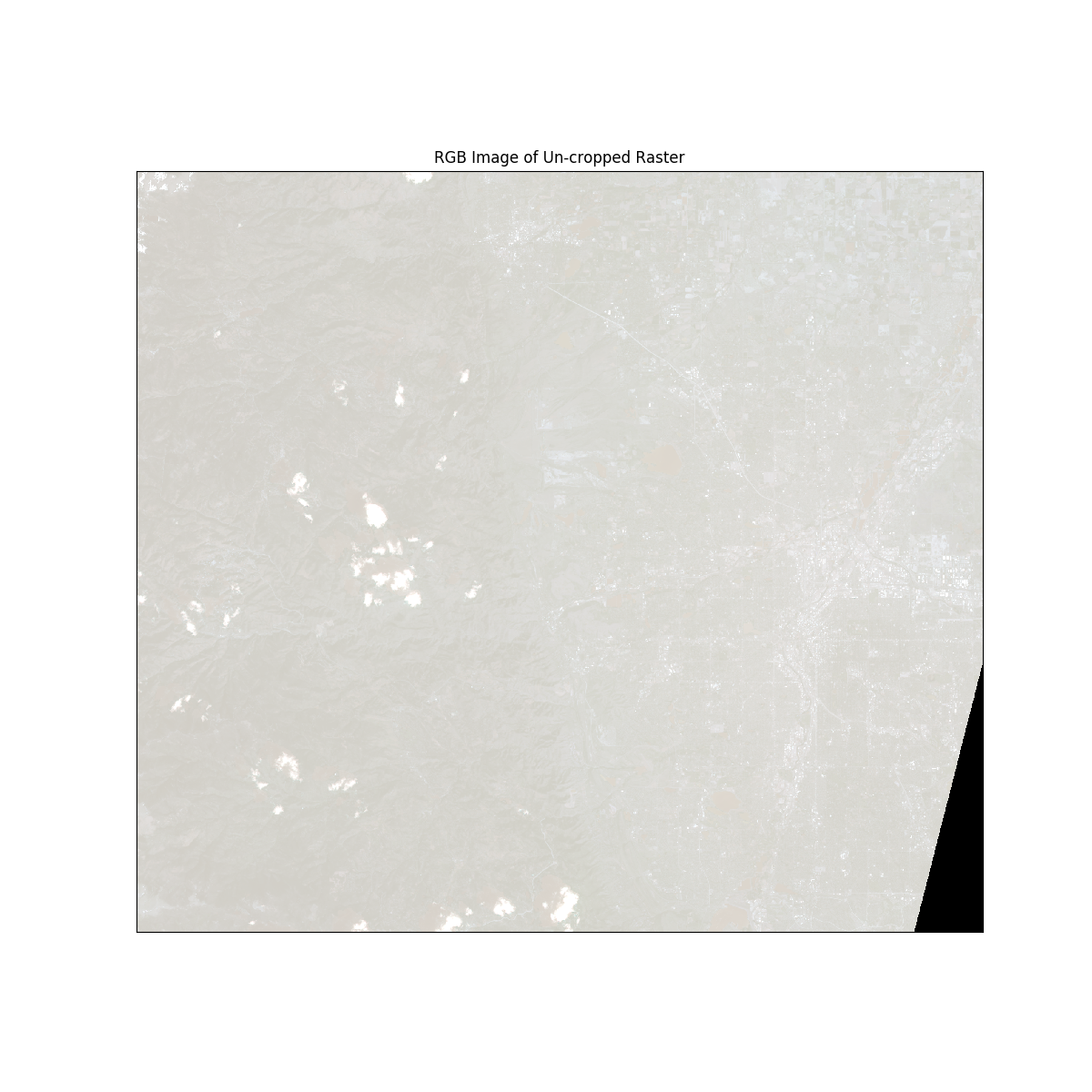
Plot Un-cropped Data
You can see the boundary and the raster before the crop using ep.plot_rgb()
Notice that the data appear washed out.
fig, ax = plt.subplots(figsize=(12, 12))
ep.plot_rgb(
    array,
    ax=ax,
    stretch=True,
    extent=extent,
    str_clip=0.5,
    title="RGB Image of Un-cropped Raster",
)
plt.show()
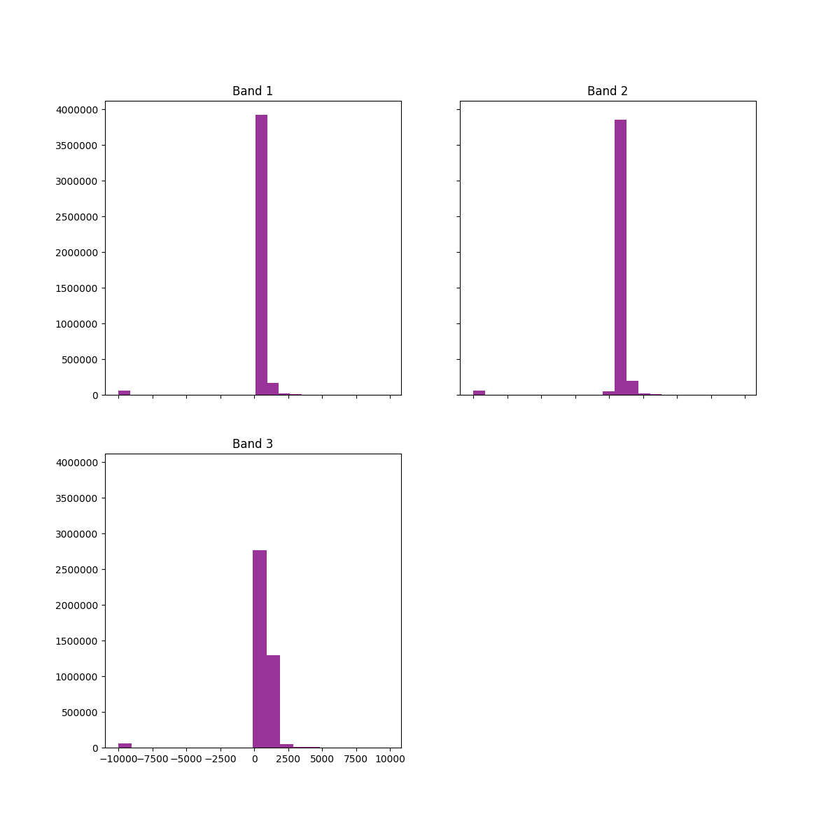
Explore the Range of Values in the Data
You can explore the range of values found in the data using the EarthPy hist()
function. Do you notice any extreme values that may be impacting the stretch
of the image?
ep.hist(array, title=["Band 1", "Band 2", "Band 3"])
plt.show()
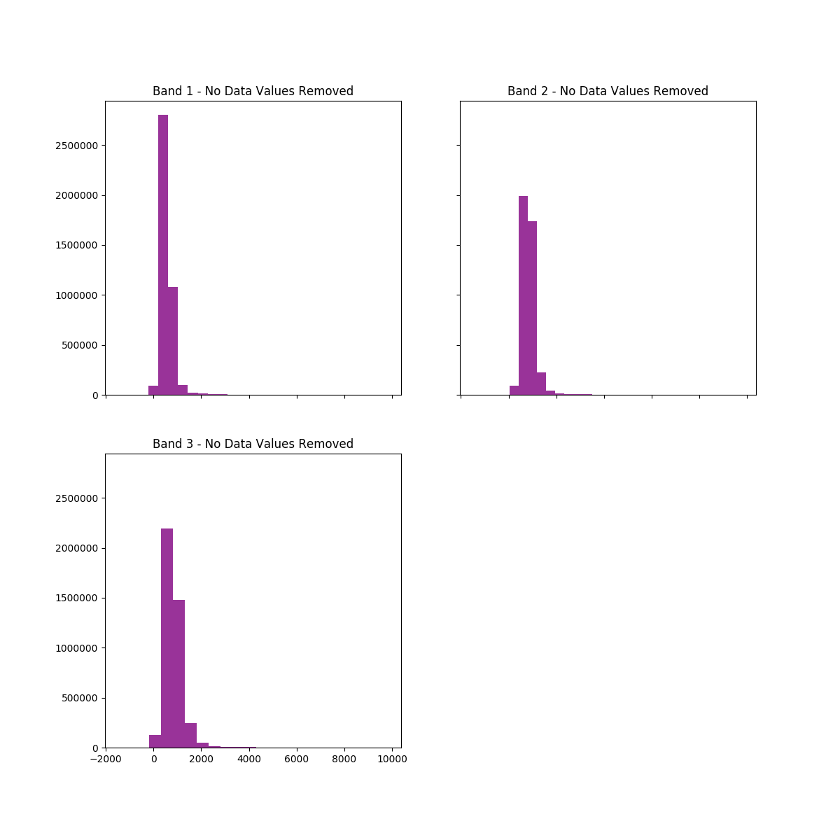
No Data Option
es.stack() can handle nodata values in a raster. To use this
parameter, specify nodata=. This will mask every pixel that contains
the specified nodata value. The output will be a numpy masked array.
os.chdir(os.path.join(et.io.HOME, "earth-analytics"))
array_nodata, raster_prof_nodata = es.stack(stack_band_paths, nodata=-9999)

# View hist of data with nodata values removed
ep.hist(
    array_nodata,
    title=[
        "Band 1 - No Data Values Removed",
        "Band 2 - No Data Values Removed",
        "Band 3 - No Data Values Removed",
    ],
)
plt.show()

# Recreate extent object for the No Data array

extent_nodata = plotting_extent(
    array_nodata[0], raster_prof_nodata["transform"]
)
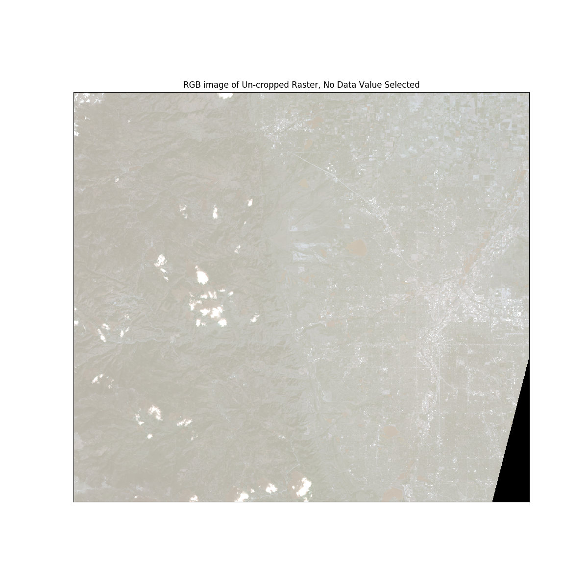
Plot Un-cropped Data
Plot the data again after the nodata values are removed.
fig, ax = plt.subplots(figsize=(12, 12))
ep.plot_rgb(
    array_nodata,
    ax=ax,
    stretch=True,
    extent=extent,
    str_clip=0.5,
    title="RGB image of Un-cropped Raster, No Data Value Selected",
)
plt.show()
Crop the Data
Sometimes you have data for an area that is larger than your study area. It is more efficient to first crop the data to your study area before processing it in Python. The fastest and most efficient option is to crop each file individually, write out the cropped raster to a new file, and then stack the new files together. To do this, make sure you have a ShapeFile boundary in the form of a GeoPandas object you can use as the cropping object. Then, loop through every file you wish to crop and crop the image, then write it out to a file. Take the rasters created and stack them like you stacked bands in the previous examples.
os.chdir(os.path.join(et.io.HOME, "earth-analytics"))

# Open the crop boundary using GeoPandas.

crop_bound = gpd.read_file(
    "data/vignette-landsat/vector_layers/fire-boundary-geomac/co_cold_springs_20160711_2200_dd83.shp"
)
Reproject the data
Note
If you are on windows, make sure to set your environment here!
The crop function won’t work properly if the data are in different Coordinate
Reference Systems (CRS). To fix this, be sure to reproject the crop layer to match
the CRS of your raster data.
To reproject your data, first get the CRS of the raster from the rasterio profile
object. Then use that to reproject using geopandas .to_crs method.
os.chdir(os.path.join(et.io.HOME, "earth-analytics"))

with rio.open(stack_band_paths[0]) as raster_crs:
    crop_raster_profile = raster_crs.profile
    crop_bound_utm13N = crop_bound.to_crs(crop_raster_profile["crs"])
Crop Each Band
When you need to crop and stack a set of images, it is most efficient to first crop each image, and then stack it. es.crop_all() is an efficient way to crop all bands in an image quickly. The function will write out cropped rasters to a directory and return a list of file paths that can then be used with es.stack().
os.chdir(os.path.join(et.io.HOME, "earth-analytics"))

band_paths_list = es.crop_all(
    stack_band_paths, output_dir, crop_bound_utm13N, overwrite=True
)
Stack All Bands
Once the data are cropped, you are ready to create a new stack.
os.chdir(os.path.join(et.io.HOME, "earth-analytics"))
cropped_array, array_raster_profile = es.stack(band_paths_list, nodata=-9999)
crop_extent = plotting_extent(
cropped_array[0], array_raster_profile["transform"]
)
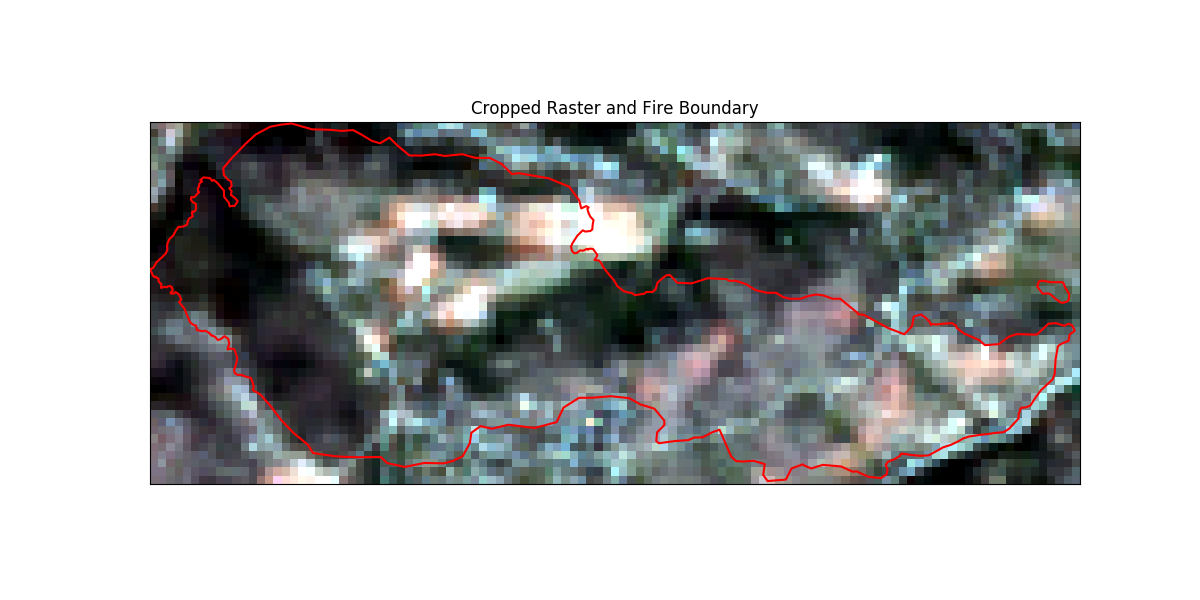
# Plotting the cropped image
# sphinx_gallery_thumbnail_number = 5
fig, ax = plt.subplots(figsize=(12, 6))
crop_bound_utm13N.boundary.plot(ax=ax, color="red", zorder=10)
ep.plot_rgb(
cropped_array,
ax=ax,
stretch=True,
extent=crop_extent,
title="Cropped Raster and Fire Boundary",
)
plt.show()
Total running time of the script: ( 0 minutes 4.591 seconds)