earthpy package

Submodules

earthpy.clip module

A module to clip vector data using geopandas

earthpy.clip.clip_shp(shp, clip_obj)

Clip points, lines, or polygon geometries to the clip_obj extent.

Both layers must be in the same Coordinate Reference System (CRS) and will be clipped to the full extent of the clip object.

If there are multiple polygons in clip_obj, data from shp will be clipped to the total boundary of all polygons in clip_obj.

Parameters:

• shp (GeoDataFrame) – Vector layer (point, line, polygon) to be clipped to clip_obj.
• clip_obj (GeoDataFrame) – Polygon vector layer used to clip shp. The clip_obj’s geometry is dissolved into one geometric feature and intersected with shp.

Returns:

Vector data (points, lines, polygons) from shp clipped to polygon boundary from clip_obj.

Return type:

GeoDataFrame

Examples

Clipping points (glacier locations in the state of Colorado) with a polygon (the boundary of Rocky Mountain National Park):

>>> import geopandas as gpd
>>> import earthpy.clip as cl
>>> from earthpy.io import path_to_example
>>> rmnp = gpd.read_file(path_to_example('rmnp.shp'))
>>> glaciers = gpd.read_file(path_to_example('colorado-glaciers.geojson'))
>>> glaciers.shape
(134, 2)
>>> rmnp_glaciers = cl.clip_shp(glaciers, rmnp)
>>> rmnp_glaciers.shape
(36, 2)

Clipping a line (the Continental Divide Trail) with a polygon (the boundary of Rocky Mountain National Park):

>>> cdt = gpd.read_file(path_to_example('continental-div-trail.geojson'))
>>> rmnp_cdt_section = cl.clip_shp(cdt, rmnp)
>>> cdt['geometry'].length > rmnp_cdt_section['geometry'].length
0    True
dtype: bool

Clipping a polygon (Colorado counties) with another polygon (the boundary of Rocky Mountain National Park):

>>> counties = gpd.read_file(path_to_example('colorado-counties.geojson'))
>>> counties.shape
(64, 13)
>>> rmnp_counties = cl.clip_shp(counties, rmnp)
>>> rmnp_counties.shape
(4, 13)

earthpy.io module

File Input/Output utilities.

class earthpy.io.Data(path=None)

Bases: object

Data storage and retrieval functionality for Earthlab.

An object of this class is available upon importing earthpy as earthpy.data that writes data files to the path: ~/earth-analytics/data/.

Parameters:path (string | None) – The path where data is stored. NOTE: this defaults to the directory ~/earth-analytics/data/.

Examples

List datasets that are available for download, using default object:

>>> import earthpy as et
>>> et.data
Available Datasets: ['california-rim-fire', ...]

Specify a custom directory for data downloads:

>>> et.data.path = "."
>>> et.data
Available Datasets: ['california-rim-fire', ...]

get_data(key=None, url=None, replace=False, verbose=True)

Retrieve the data for a given week and return its path.

This will retrieve data from the internet if it isn’t already downloaded, otherwise it will only return a path to that dataset.

Parameters:

• key (str) – The dataset to retrieve. Possible options can be found in self.data_keys. Note: key and url are mutually exclusive.
• url (str) – A URL to fetch into the data directory. Use this for ad-hoc dataset downloads. Note: key and url are mutually exclusive.
• replace (bool) – Whether to replace the data for this key if it is already downloaded.
• verbose (bool) – Whether to print verbose output while downloading files.

Returns:

path_data – The path to the downloaded data.

Return type:

str

Examples

Download a dataset using a key:

>>> et.data.get_data('california-rim-fire') # doctest: +SKIP

Or, download a dataset using a figshare URL:

>>> url = 'https://ndownloader.figshare.com/files/12395030'
>>> et.data.get_data(url=url)  # doctest: +SKIP

earthpy.io.path_to_example(dataset)

Construct a file path to an example dataset.

This file defines helper functions to access data files in this directory, to support examples. Adapted from the PySAL package.

Parameters:dataset (string) – Name of a dataset to access (e.g., “epsg.json”, or “RGB.byte.tif”) Returns: Return type:A file path (string) to the dataset

Example

>>> import earthpy.io as eio
>>> eio.path_to_example('rmnp-dem.tif')
'...rmnp-dem.tif'

earthpy.mask module

earthpy.mask.mask_pixels(arr, mask_arr, vals=None)

Apply a mask to an input array.

Masks values in an n-dimensional input array (arr) based on input 1-dimensional array (mask_arr). If mask_arr is provided in a boolean format, it is used as a mask. If mask_arr is provided as a non-boolean format and values to mask (vals) are provided, a Boolean masked array is created from the mask_arr and the indicated vals to mask, and then this new 1-dimensional masked array is used to mask the input arr.

This function is useful when masking cloud and other unwanted pixels.

Parameters:

• arr (numpy array) – The array to mask in rasterio (band, row, col) order.
• mask_arr (numpy array) – An array of either the pixel_qa or mask of interest.
• vals (list of numbers either int or float (optional)) – A list of values from the pixel qa layer that will be used to create the mask for the final return array. If vals are not passed in, it is assumed the mask_arr given is the mask of interest.

Returns:

arr – A numpy array populated with 1’s where the mask is applied (a Boolean True) and the original numpy array’s value where no masking was done.

Return type:

numpy array

Example

>>> import numpy as np
>>> from earthpy.mask import mask_pixels
>>> im = np.arange(9).reshape((3, 3))
>>> im
array([[0, 1, 2],
       [3, 4, 5],
       [6, 7, 8]])
>>> im_mask = np.array([1, 1, 1, 0, 0, 0, 1, 1, 1]).reshape(3, 3)
>>> im_mask
array([[1, 1, 1],
       [0, 0, 0],
       [1, 1, 1]])
>>> mask_pixels(im, mask_arr=im_mask, vals=[1])
masked_array(
  data=[[--, --, --],
        [3, 4, 5],
        [--, --, --]],
  mask=[[ True,  True,  True],
        [False, False, False],
        [ True,  True,  True]],
  fill_value=999999)

earthpy.plot module

The earthpy spatial module provides functions that wrap around rasterio and geopandas to work with raster and vector data in Python.

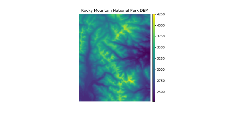
earthpy.plot.colorbar(mapobj, size='3%', pad=0.09)

Adjust colorbar height to match the matplotlib axis height.

NOTE: This function requires matplotlib v 3.0.1 or greater or v 2.9 or lower to run properly.

Parameters:

• mapobj (matplotlib axis object) – The image that the colorbar will be representing as a matplotlib axis object.
• size (char (default = "3%")) – The percent width of the colorbar relative to the plot.
• pad (int (default = 0.09)) – The space between the plot and the color bar.

Returns:

Matplotlib color bar object with the correct width that matches the y-axis height.

Return type:

matplotlib.pyplot.colorbar

Examples

>>> import matplotlib.pyplot as plt
>>> import rasterio as rio
>>> import earthpy.plot as ep
>>> from earthpy.io import path_to_example
>>> with rio.open(path_to_example('rmnp-dem.tif')) as src:
...     dem = src.read()
...     fig, ax = plt.subplots(figsize = (10, 5))
>>> im = ax.imshow(dem.squeeze())
>>> ep.colorbar(im)
<matplotlib.colorbar.Colorbar object at 0x...>
>>> ax.set(title="Rocky Mountain National Park DEM")
[Text(...'Rocky Mountain National Park DEM')]
>>> ax.set_axis_off()
>>> plt.show()

(Source code, png, hires.png, pdf)

earthpy.plot.draw_legend(im_ax, bbox=(1.05, 1), titles=None, cmap=None, classes=None)

Create a custom legend with a box for each class in a raster.

Parameters:

• im_ax (matplotlib image object) – This is the image returned from a call to imshow().
• bbox (tuple (default = (1.05, 1))) – This is the bbox_to_anchor argument that will place the legend anywhere on or around your plot.
• titles (list (optional)) – A list of a title or category for each unique value in your raster. This is the label that will go next to each box in your legend. If nothing is provided, a generic “Category x” will be populated.
• cmap (str (optional)) – Colormap name to be used for legend items.
• classes (list (optional)) – A list of unique values found in the numpy array that you wish to plot.

Returns:

A matplotlib legend object to be placed on the plot.

Return type:

matplotlib.pyplot.legend

Example

>>> import numpy as np
>>> import earthpy.plot as ep
>>> import matplotlib.pyplot as plt
>>> im_arr = np.random.uniform(-2, 1, (15, 15))
>>> bins = [-np.Inf, -0.8, 0.8, np.Inf]
>>> im_arr_bin = np.digitize(im_arr, bins)
>>> cat_names = ["Class 1", "Class 2", "Class 3"]
>>> f, ax = plt.subplots()
>>> im = ax.imshow(im_arr_bin, cmap="gnuplot")
>>> im_ax = ax.imshow(im_arr_bin)
>>> leg_neg = ep.draw_legend(im_ax = im_ax, titles = cat_names)

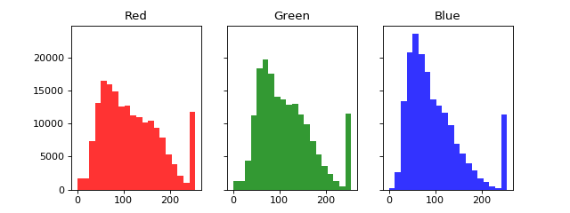
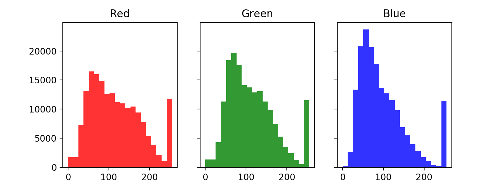
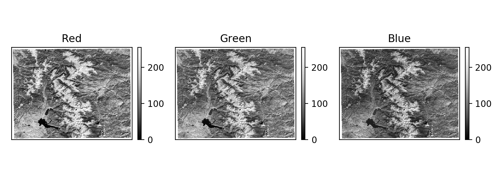
earthpy.plot.hist(arr, colors=['purple'], figsize=(12, 12), cols=2, bins=20, title=None)

Plot histogram for each layer in a numpy array.

Parameters:

• arr (numpy array) – An n-dimensional numpy array from which n histograms will be plotted.
• colors (list (default = ["purple"])) – A list of color values that should either equal the number of bands or be a single color.
• figsize (tuple (default = (12, 12))) – The x and y integer dimensions of the output plot.
• cols (int (default = 2)) – The number of columns for plot grid.
• bins (int (default = 20)) – The number of bins to generate for the histogram.
• title (list (optional)) – A list of title values that should either equal the number of bands or be empty.

Returns:

fig : figure object

The figure object associated with the histogram.

ax or axs : ax or axes object

The axes object(s) associated with the histogram.

Return type:

tuple

Example

>>> import matplotlib.pyplot as plt
>>> import rasterio as rio
>>> import earthpy.plot as ep
>>> from earthpy.io import path_to_example
>>> with rio.open(path_to_example('rmnp-rgb.tif')) as src:
...     img_array = src.read()
>>> ep.hist(img_array,
...     colors=['r', 'g', 'b'],
...     title=['Red', 'Green', 'Blue'],
...     cols=3,
...     figsize=(8, 3))
(<Figure size 800x300 with 3 Axes>, ...)

(Source code, png, hires.png, pdf)

earthpy.plot.make_col_list(unique_vals, nclasses=None, cmap=None)

Convert a matplotlib named colormap into a discrete list of n-colors in RGB format.

Parameters:

• unique_vals (list) – A list of values to make a color list from.
• nclasses (int (optional)) – The number of classes.
• cmap (str (optional)) – Colormap name used to create output list.

Returns:

A list of colors based on the given set of values in matplotlib format.

Return type:

list

Example

>>> import numpy as np
>>> import earthpy.plot as ep
>>> import matplotlib.pyplot as plt
>>> arr = np.array([[1, 2], [3, 4], [5, 4], [5, 5]])
>>> f, ax = plt.subplots()
>>> im = ax.imshow(arr, cmap="Blues")
>>> the_legend = ep.draw_legend(im_ax=im)
>>> # Get the array and cmap from axis object
>>> cmap_name = im.axes.get_images()[0].get_cmap().name
>>> unique_vals = list(np.unique(im.get_array().data))
>>> cmap_colors = ep.make_col_list(unique_vals, cmap=cmap_name)

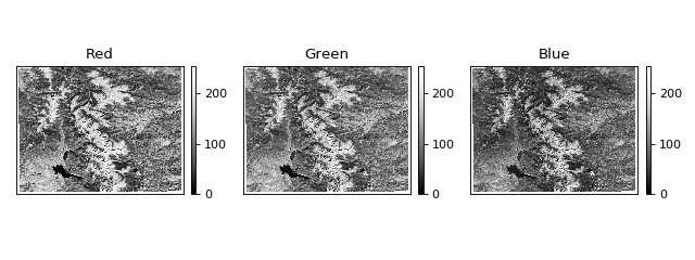
earthpy.plot.plot_bands(arr, cmap='Greys_r', figsize=(12, 12), cols=3, title=None, extent=None, cbar=True, scale=True, vmin=None, vmax=None)

Plot each band in a numpy array in its own axis.

Assumes band order (band, row, col).

Parameters:

• arr (numpy array) – An n-dimensional numpy array to plot.
• cmap (str (default = "Greys_r")) – Colormap name for plots.
• figsize (tuple (default = (12, 12))) – Figure size in inches.
• cols (int (default = 3)) – Number of columns for plot grid.
• title (str or list (optional)) – Title of one band or list of titles with one title per band.
• extent (tuple (optional)) – Bounding box that the data will fill: (minx, miny, maxx, maxy).
• cbar (Boolean (default = True)) – Turn off colorbar if needed.
• scale (Boolean (Default = True)) – Turn off bytescale scaling if needed.
• vmin (Int (Optional)) – Specify the vmin to scale imshow() plots.
• vmax (Int (Optional)) – Specify the vmax to scale imshow() plots.

Returns:

fig : figure object

The figure of the plotted band(s).

ax or axs : axes object(s)

The axes object(s) associated with the plot.

Return type:

tuple

Example

>>> import matplotlib.pyplot as plt
>>> import earthpy.plot as ep
>>> from earthpy.io import path_to_example
>>> import rasterio as rio
>>> titles = ['Red', 'Green', 'Blue']
>>> with rio.open(path_to_example('rmnp-rgb.tif')) as src:
...     ep.plot_bands(src.read(),
...                   title=titles,
...                   figsize=(8, 3))
array([<matplotlib.axes._subplots.AxesSubplot object at 0x...

(Source code, png, hires.png, pdf)

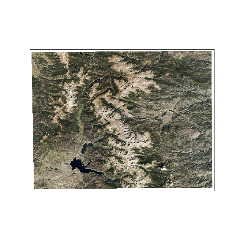
earthpy.plot.plot_rgb(arr, rgb=(0, 1, 2), figsize=(10, 10), str_clip=2, ax=None, extent=None, title='', stretch=None)

Plot three bands in a numpy array as a composite RGB image.

Parameters:

• arr (numpy array) – An n-dimensional array in rasterio band order (bands, rows, columns) containing the layers to plot.
• rgb (list (default = (0, 1, 2))) – Indices of the three bands to be plotted.
• figsize (tuple (default = (10, 10)) – The x and y integer dimensions of the output plot.
• str_clip (int (default = 2)) – The percentage of clip to apply to the stretch. Default = 2 (2 and 98).
• ax (object (optional)) – The axes object where the ax element should be plotted.
• extent (tuple (optional)) – The extent object that matplotlib expects (left, right, bottom, top).
• title (string (optional)) – The intended title of the plot.
• stretch (Boolean (optional)) – Application of a linear stretch. If set to True, a linear stretch will be applied.

Returns:

fig : figure object

The figure object associated with the 3 band image. If the ax keyword is specified, the figure return will be None.

ax : axes object

The axes object associated with the 3 band image.

Return type:

tuple

Example

>>> import matplotlib.pyplot as plt
>>> import rasterio as rio
>>> import earthpy.plot as ep
>>> from earthpy.io import path_to_example
>>> with rio.open(path_to_example('rmnp-rgb.tif')) as src:
...     img_array = src.read()
>>> ep.plot_rgb(img_array)
(<Figure size 1000x1000 with 1 Axes>, ...)

(Source code, png, hires.png, pdf)

earthpy.spatial module

The earthpy spatial module provides functions that wrap around rasterio and geopandas to make it easier to manipulate raster raster and vector data in Python.

earthpy.spatial.bytescale(data, high=255, low=0, cmin=None, cmax=None)

Byte scales an array (image).

Byte scaling converts the input image to uint8 dtype, and rescales the data range to (low, high) (default 0-255). If the input image already has dtype uint8, no scaling is done. Source code adapted from scipy.misc.bytescale (deprecated in scipy-1.0.0)

Parameters:

• data (numpy array) – image data array.
• high (int (default=255)) – Scale max value to high.
• low (int (default=0)) – Scale min value to low.
• cmin (int (optional)) – Bias scaling of small values. Default is data.min().
• cmax (int (optional)) – Bias scaling of large values. Default is data.max().

Returns:

img_array – The byte-scaled array.

Return type:

uint8 numpy array

Examples

>>> import numpy as np
>>> from earthpy.spatial import bytescale
>>> img = np.array([[ 91.06794177,   3.39058326,  84.4221549 ],
...                 [ 73.88003259,  80.91433048,   4.88878881],
...                 [ 51.53875334,  34.45808177,  27.5873488 ]])
>>> bytescale(img)
array([[255,   0, 236],
       [205, 225,   4],
       [140,  90,  70]], dtype=uint8)
>>> bytescale(img, high=200, low=100)
array([[200, 100, 192],
       [180, 188, 102],
       [155, 135, 128]], dtype=uint8)
>>> bytescale(img, cmin=0, cmax=255)
array([[255,   0, 236],
       [205, 225,   4],
       [140,  90,  70]], dtype=uint8)

earthpy.spatial.crop_image(raster, geoms, all_touched=True)

Crop a single file using geometry objects.

Parameters:

• raster (rasterio object) – The rasterio object to be cropped.
• geoms (geopandas geodataframe or list of polygons) – The spatial polygon boundaries in GeoJSON-like dict format to be used to crop the image. All data outside of the polygon boundaries will be set to nodata and/or removed from the image.
• all_touched (bool (default=True)) – Include a pixel in the mask if it touches any of the shapes. If False, include a pixel only if its center is within one of the shapes, or if it is selected by Bresenham’s line algorithm. (from rasterio)

Returns:

out_image: cropped numpy array

A numpy array that is cropped to the geoms object extent with shape (bands, rows, columns)

out_meta: dict

A dictionary containing updated metadata for the cropped raster, including extent (shape elements) and transform properties.

Return type:

tuple

Example

>>> import geopandas as gpd
>>> import rasterio as rio
>>> import earthpy.spatial as es
>>> from earthpy.io import path_to_example
>>> # Clip an RGB image to the extent of Rocky Mountain National Park
>>> rmnp = gpd.read_file(path_to_example("rmnp.shp"))
>>> with rio.open(path_to_example("rmnp-rgb.tif")) as raster:
...     src_image = raster.read()
...     out_image, out_meta = es.crop_image(raster, rmnp)
>>> out_image.shape
(3, 265, 281)
>>> src_image.shape
(3, 373, 485)

earthpy.spatial.extent_to_json(ext_obj)

Convert bounds to a shapely geojson like spatial object.

This format is what shapely uses. The output object can be used to crop a raster image.

Parameters:ext_obj (list or geopandas geodataframe) – If provided with a geopandas geodataframe, the extent will be generated from that. Otherwise, extent values should be in the order: minx, miny, maxx, maxy. Returns:

• extent_json (A GeoJSON style dictionary of corner coordinates)
• for the extent – A GeoJSON style dictionary of corner coordinates representing the spatial extent of the provided spatial object.

Example

>>> import geopandas as gpd
>>> import earthpy.spatial as es
>>> from earthpy.io import path_to_example
>>> rmnp = gpd.read_file(path_to_example('rmnp.shp'))
>>> es.extent_to_json(rmnp)
{'type': 'Polygon', 'coordinates': (((-105.4935937, 40.1580827), ...),)}

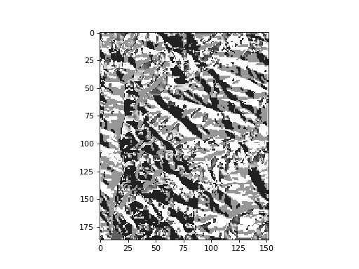
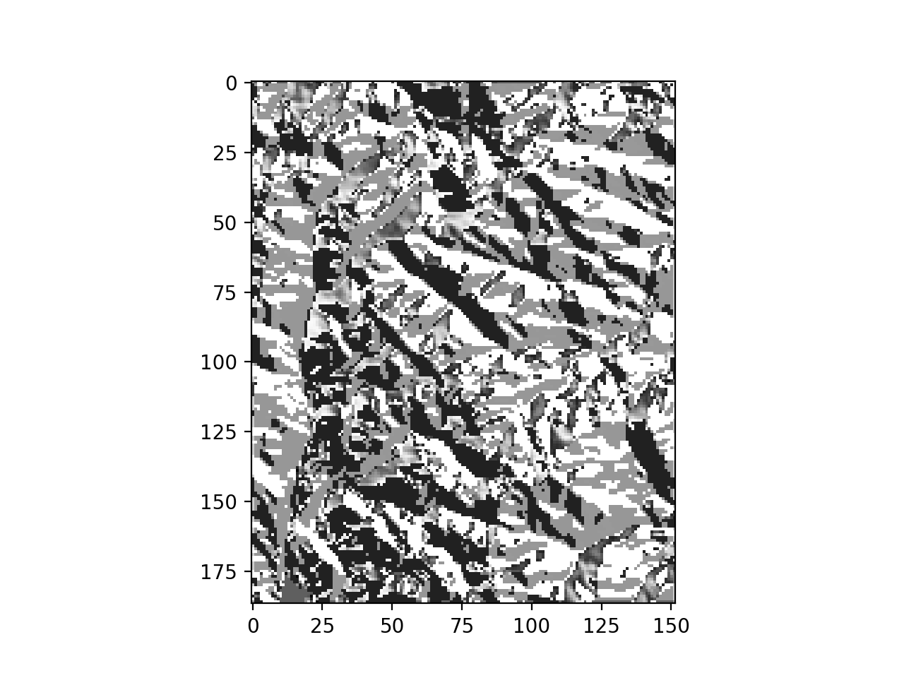
earthpy.spatial.hillshade(arr, azimuth=30, angle_altitude=30)

Create hillshade from a numpy array containing elevation data.

Parameters:

• arr (numpy array of shape (rows, columns)) – Numpy array containing elevation values to be used to created hillshade.
• azimuth (float (default=30)) – The desired azimuth for the hillshade.
• angle_altitude (float (default=30)) – The desired sun angle altitude for the hillshade.

Returns:

A numpy array containing hillshade values.

Return type:

numpy array

Example

>>> import matplotlib.pyplot as plt
>>> import rasterio as rio
>>> import earthpy.spatial as es
>>> from earthpy.io import path_to_example
>>> with rio.open(path_to_example('rmnp-dem.tif')) as src:
...     dem = src.read()
>>> print(dem.shape)
(1, 187, 152)
>>> squeezed_dem = dem.squeeze() # remove first dimension
>>> print(squeezed_dem.shape)
(187, 152)
>>> shade = es.hillshade(squeezed_dem)
>>> plt.imshow(shade, cmap="Greys")
<matplotlib.image.AxesImage object at 0x...>

(Source code, png, hires.png, pdf)

earthpy.spatial.normalized_diff(b1, b2)

Take two n-dimensional numpy arrays and calculate the normalized difference.

Math will be calculated (b1-b2) / (b1 + b2).

Parameters:b2 (b1,) – Two numpy arrays that will be used to calculate the normalized difference. Math will be calculated (b1-b2) / (b1+b2). Returns:n_diff – The element-wise result of (b1-b2) / (b1+b2) calculation. Inf values are set to nan. Array returned as masked if result includes nan values. Return type:numpy array

Examples

>>> import numpy as np
>>> import earthpy.spatial as es
>>> # Calculate normalized difference vegetation index
>>> nir_band = np.array([[6, 7, 8, 9, 10], [16, 17, 18, 19, 20]])
>>> red_band = np.array([[1, 2, 3, 4, 5], [11, 12, 13, 14, 15]])
>>> ndvi = es.normalized_diff(b1=nir_band, b2=red_band)
>>> ndvi
array([[0.71428571, 0.55555556, 0.45454545, 0.38461538, 0.33333333],
       [0.18518519, 0.17241379, 0.16129032, 0.15151515, 0.14285714]])

>>> # Calculate normalized burn ratio
>>> nir_band = np.array([[8, 10, 13, 17, 15], [18, 20, 22, 23, 25]])
>>> swir_band = np.array([[6, 7, 8, 9, 10], [16, 17, 18, 19, 20]])
>>> nbr = es.normalized_diff(b1=nir_band, b2=swir_band)
>>> nbr
array([[0.14285714, 0.17647059, 0.23809524, 0.30769231, 0.2       ],
       [0.05882353, 0.08108108, 0.1       , 0.0952381 , 0.11111111]])

earthpy.spatial.stack(band_paths, out_path='')

Convert a list of raster paths into a raster stack numpy darray.

Parameters:

• band_paths (list of file paths) – A list with paths to the bands to be stacked. Bands will be stacked in the order given in this list.
• out_path (string (optional)) – A path with a file name for the output stacked raster tif file.

Returns:

numpy array

N-dimensional array created by stacking the raster files provided.

rasterio profile object

A rasterio profile object containing the updated spatial metadata for the stacked numpy array.

Return type:

tuple

Example

>>> import os
>>> import earthpy.spatial as es
>>> from earthpy.io import path_to_example
>>> band_fnames = ["red.tif", "green.tif", "blue.tif"]
>>> band_paths = [path_to_example(fname) for fname in band_fnames]
>>> destfile = "./stack_result.tif"
>>> arr, arr_meta = es.stack(band_paths, destfile)
>>> arr.shape
(3, 373, 485)
>>> os.path.isfile(destfile)
True
>>> # optionally, clean up example output
>>> os.remove(destfile)

earthpy.spatial.stack_raster_tifs(band_paths, out_path, arr_out=True)

This function has been deprecated from earthpy.

Please use the stack() function instead.

Module contents

Utility functions for the working with spatial data.

earthpy.load_epsg()

A function to return a dictionary of EPSG code to Proj4 string mappings.

This function supports calling epsg[‘code-here’].

Returns:epsg – The epsg dictionary contains mappings of EPSG integer string codes to Proj4 strings. Return type:dictionary

Example

>>> import earthpy as et
>>> # Get Proj4 string for EPSG code 4326
>>> et.epsg['4326']
'+proj=longlat +datum=WGS84 +no_defs'